Chapter 4: Multitaper Spectral Analysis of High-frequency Seismograms: Figures

• Title
• Abstract
• Chapter 1
• Chapter 2
• Chapter 3
• Chapter 4
• Chapter 5
• Chapter 6
• Figures
• Chapter 1
• Chapter 2
• Chapter 3
• Chapter 4
• Chapter 5
• Chapter 6

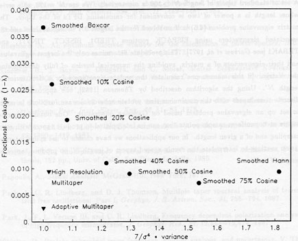
Figure 1

Comparison plot of boxcar, Hann, and 20% cosine tapers.

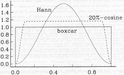
Figure 2

The five lowest-order 4π prolate eigentapers. The zeroth-order eigentaper v⁽⁰⁾ is plotted with a solid line, and the higher-order tapers are plotted with dashed lines.

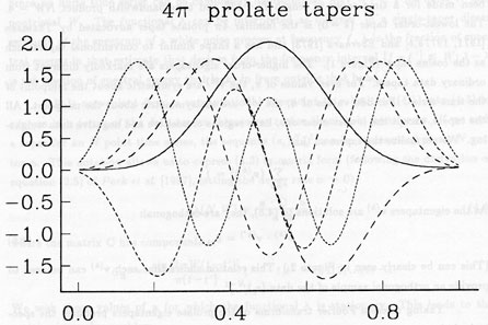
Figure 3

Fourier transform amplitudes of the five 4π prolate tapers shown in Figure 2, using the same conventions for dashed and solid lines.

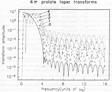
Figure 4

(Top panel, between dashed vertical lines) Comparison of unsmoothed and smoothed estimates of the spectrum of a high-frequency S wave. The spectra are plotted on a log-linear scale and are offset to facilitate comparison. The boxcar spectral estimates are graphed with a solid line. The dashed lines at the top of each of the lower figures are spectral estimates employing a Hann taper. The middle curves are spectral estimates obtained using a 20% cosine taper.

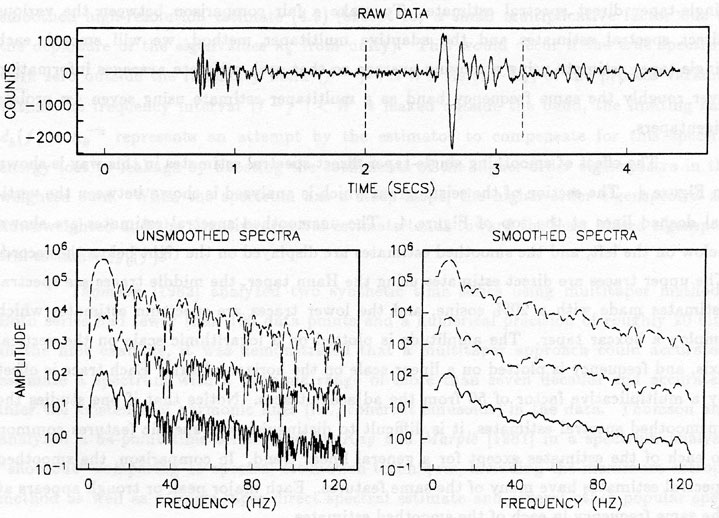
Figure 5

A multitaper spectral estimate (solid line, labeled a) of the frequency content of an SH wave (top, between vertical dashed lines) is compared with direct spectral estimates using the boxcar taper (fine dashed line, labeled b), 20% cosine taper (coarse dashed line, labeled c), and Hann taper (asterisks, labeled d). The spectra are plotted using linear scales for the horizontal and vertical axes. The boxcar, 20% cosine, and multitaper estimates of the S wave spectrum are almost identical, but the Hann taper estimate is substantially different. This is because the Hann-tapered spectra overemphasize the data in the center of the time series and downweight data points toward the ends of the record. The section of the time series which was analyzed is bracketed by dashed lines in the seismogram at the top.

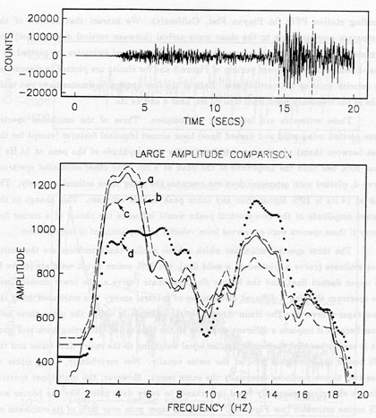
Figure 6

Comparison of the leakage of various estimates of the spectrum of a vertical seismogram recorded 412 km away from a Nevada Test Site explosion. The spectral estimate using a cosine taper (asterisks, labeled d) and the multitaper spectral estimate (solid line, labeled a) give good representations of the spectra of the seismic signal (0 -20 Hz) and ground noise (20 -60 Hz). The spectra are plotted using a log-linear scale.

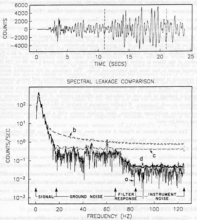
Figure 7

Comparison of the variance and broadband bias of several single-taper spectral estimates (solid circles) and the multitaper estimates (solid triangles).